Shortwave Direction finding

Operation RAFTER

RAFTER was a code name for the MI5 radio receiver detection technique, mostly used against clandestine Soviet agents and monitoring of domestic radio transmissions by foreign embassy personnel from the 1950s on.

Explanation

Since most radio receivers are of the superhet design, they typically contain local oscillators which generate a radio frequency signal in the range of 455 kHz above or sometimes below the frequency to be received. There is always some radiation from such receivers, and in the initial stages of RAFTER, MI5 simply attempted to locate clandestine receivers based on picking up the superhet signal with a quiet sensitive receiver that was custom built. This was not always easy because of the increasing number of domestic radios and televisions in people's homes.

By accident, one such receiver for MI5 mobile radio transmissions was being monitored when a passing transmitter produced a powerful signal. This overloaded the receiver, producing an audible change in the received signal. Quickly the agency realized that they could identify the actual frequency being monitored if they produced their own transmissions and listened for the change in the superhet tone.


Soviet transmitters

Since Soviet short-wave transmitters were extensively used to broadcast messages to clandestine agents, the transmissions consisting simply of number sequences read aloud and decoded using a one-time pad, it was realized that this new technique could be used to track down such agents. Specially equipped aircraft would fly over urban areas at times when the Soviets were transmitting, and attempt to locate receivers tuned to the Soviet transmissions.


Tactics

Like many secret technologies, RAFTER's use was attended by the fear of over-use, alerting the quarry and causing a shift in tactics which would neutralize the technology. As a technical means of intelligence, it was also not well supported by the more traditional factions in MI5. Its part in the successes and failures of MI5 at the time is not entirely known.

In his book Spycatcher[1] , MI5 officer Peter Wright related one incident in which a mobile RAFTER unit in a van, or panel truck, was driven around the backstreets in an attempt to locate a receiver. What with interference and the effects of large metal objects in the surroundings, such as lamp posts, this proved futile. Later, however, they concluded that the receiver itself had been mobile, and may at one point have been parked next to the van, hidden by a high fence.


References

   1. ^ Spycatcher: The Autobiography of a Senior Intelligence Officer, by Peter Wright, 1987.

High frequency direction finding, usually known by its abbreviation HF/DF (nicknamed



huff-duff, pronounced "aitch eff dee eff") is the common name for a type of radio direction finding employed especially during the two World Wars.

The idea of using two or more radio receivers to find the bearings of a radio transmitter and with the use of simple triangulation find the approximate position of the transmitter had been known and used since the invention of wireless communication. The general principle is to rotate a directional aerial and note where the signal is strongest. With simple aerial design the signal will be strongest when pointing directly towards and directly away from the source, so two bearings from different positions are usually taken, and the intersection plotted. More modern aerials employ uni-directional techniques.

HF/DF was used by early aviators to obtain bearings of radio transmitters at airfields by rotatable aerials above the cockpit, and during World War I shore installations of all protagonists endeavoured to obtain information about ship movements in this way. The requirement both to tune a radio and rotate an aerial manually made this a cumbersome and slow business, and one which could be evaded if the radio transmission were short enough. Films depicting World War II spies transmitting covertly will sometimes show detection vans attached to patrols performing this activity.

Finding the location of radio and radar transmitters is one of the fundamental disciplines of Signal Intelligence SIGINT. In the World War II context, Huff Duff applied to direction-finding of radio communications transmitters, typically operating at high frequency (HF). Modern direction finding of both communications and noncommunications signals covers a much wider range of frequencies.



Within communications intelligence (COMINT), direction finding is part of the armoury of the intelligence analyst. Sister disciplines within COMINT include cryptanalysis, the analysis of the content of encrypted messages, and traffic analysis, the analysis of the patterns of senders and addressees. While it was not a significant World War II tool, there are a variety of Measurement and Signal Intelligence (MASINT) techniques that extract information from unintentional signals from transmitters, such as the oscillator frequency of a superheterodyne radio receiver.



Along with ASDIC (sonar), Ultra code breaking (COMINT) and radar, "Huff-Duff" was a valuable part of the Allies' armoury in detecting German U-boats and commerce raiders during the Battle of the Atlantic.

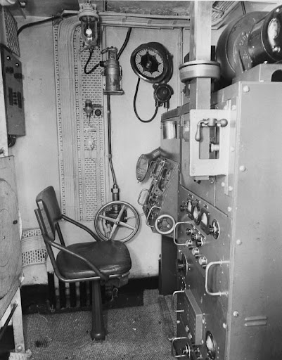
The Royal Navy designed a particularly sophisticated apparatus that could take bearings on the high frequency radio transmitters employed by the German Kriegsmarine in World War II. There were severe technical problems of engineering effective high frequency direction finding systems for operation on ships, mainly due to the effects of the superstructure on the wavefront of arriving radio signals. However, these problems were overcome under the technical leadership of the Polish engineer Waclaw Struszyn'ski, working at the Admiralty Signal Establishment.

Many shore based installations were constructed around the North Atlantic and whenever a U-boat transmitted a message, "Huff-Duff" could get bearings on the approximate position of the boat. Because it worked on the electronic emission and not the content of the message, it did not matter that the content was encrypted using an Enigma machine. This information was then transmitted to convoys at sea, and a complex chess game developed as Royal Navy controllers tried to manoeuvre wide convoys past strings of U-Boats set up by the Kriegsmarine controllers.

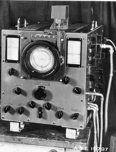
A key feature of the British "Huff-Duff" was the use of an oscilloscope display and fixed aerial which could instantaneously reveal the direction of the transmission, without the time taken in conventional direction finding to rotate the aerial -- U-boat transmissions were deliberately kept short, and it was wrongly assumed by the U-boat captains that this would avoid detection of the sender's direction.

Another feature was the use of continuously motor-driven tuning, to scan the likely frequencies to pick up and sound an automatic alarm when any transmissions were detected.

In 1942 the allies began to install Huff-Duff on convoy escort ships, enabling them to get much more accurate triangulation fixes on U-boats transmitting from over the horizon, beyond the range of radar. This allowed hunter-killer ships and aircraft to be dispatched at high speed in the direction of the U-boat, which could be illuminated by radar if still on the surface and by ASDIC if it had dived. It was the operation of these technologies in combination which eventually turned the tide against the U-boats.


Battle of Britain

During the Battle of Britain the Royal Air Force (RAF) deployed an Identification Friend or Foe (IFF) system codenamed "pipsqueak". RAF fighters had a clockwork mechanism that regulated the broadcast of a signal over an HF channel for fourteen seconds of every minute. Each Fighter Command sector had Huff-Duff receiving stations that would monitor the "pipsqueak" broadcasts and telephone the bearings back to the sector control rooms where they could be triangulated and the squadron's location plotted.



Wullenweber

The Wullenweber (the original name introduced by Dr. Hans Rindfleisch was Wullenwever) is a type of Circularly Disposed Antenna Array (CDAA) sometimes referred to as a Circularly Disposed Dipole Array (CDDA). It is a large circular antenna array used for radio direction finding. It was used by the military to triangulate radio signals for radio navigation, intelligence gathering and search and rescue. Because its huge circular reflecting screen looks like a circular fence, the antenna has been colloquially referred to as the elephant cage. Wullenwever was the World War II German cover term used to identify their CDAA research and development program; its name is unrelated to any person involved in the program.

Wullenwever technology was developed by the German navy communication research command, Nachrichtenmittelversuchskommando (NVK) and Telefunken during the early years of World War II. The inventor was NVK group leader Dr. Hans Rindfleisch, who worked after the war as a Technical Director for the northern Germany official broadcast ( Norddeutscher Rundfunk - NDR). Technical team leaders were Dr. Joachim Pietzner, Dr. Hans Schellhoss, and Dr. Maximilian Wächtler. The latter was a founder of Plath GmbH in 1954 and later a consultant to both Plath and Telefunken.

Dr. Rolf Wundt, a German antenna researcher, was one of hundreds of German scientists taken to the U.S. by the Army after the war under Operation Paperclip. He arrived in New York in March, 1947 on the same ship as Wernher Von Braun and his wife and parents. He was first employed by the U.S. Air Force, then by GT&E Sylvania Electronics Systems on Wullenweber and other antenna projects.

Although the three men retired in West Germany, some of their second-echelon technicians were taken to the USSR after the war. At least 30 Krug (Russian for circle) arrays were installed all over the Soviet Union and allied countries in the 1950s, well before the U.S. military became interested and developed their own CDAAs. Several Krugs were installed in pairs within less than 10 km kilometers of each other, apparently for radio navigation purposes. At least four Krugs were installed near Moscow; just to the north, east and south (55°27?51?N 37°22?11?E? / ?55.46408°N 37.3698°E? / 55.46408; 37.3698) of the city. The Krugs were used to track the early Sputnik satellites, using their 10 and 20 MHz beacons, and were instrumental in locating re-entry vehicles.



The first Wullenwever was built during the war at Skisby (in German: Hjörring), Denmark (57°28?39?N 10°20?04?E? / ?57.4775°N 10.33444°E? / 57.4775; 10.33444). It used forty vertical radiator elements, placed on the arc of a circle with a diameter of 120 meters. Forty reflecting elements were installed behind the radiator elements, suspended on a circular wooden support structure with a diameter of 112.5 meters. To more easily obtain true geographic bearings, the north and south elements were placed exactly on the North-South meridian. The Soviet Krug arrays also use the 40 radiator Wullenwever configuration.

The array in Skisby was extensively studied by the British, then destroyed following the war in accordance with the Geneva Convention. Dr. Wächtler arranged to have a second array built, at Telefunken expense, at Langenargen/Bodensee, for further experimentation after the war. In the years following the war, the U.S. disassembled the Langenargen/Bodensee array and brought it back to the U.S., where it became known as the "Wullenweber" array.

Professor Edgar Hayden, then a young engineer in the University of Illinois Radio Direction Finding Research Group, led the reassembly of the Wullenweber, studied the design and performance of HF/DF arrays and researched the physics of HF/DF under contract to the U.S. Navy from 1947 through 1960. His research is still used today to guide the design and site selection of HF/DF arrays. Records of his research are available in the university's archives. Hayden was later employed by Southwest Research Institute where he continued to contribute to HF direction finding technology.



Hayden led the design and development of a large Wullenweber array at the university's Bondville Road Field Station, a few miles southwest of Bondville, IL. The array consisted of a ring 120 vertical monopoles covering 2-20 MHz. Tall wood poles supported a 1,000-foot-diameter (300 m) circular screen of vertical wires located within the ring of monopoles. Due to their immense size, the location of the Bondville array (40°02?58?N 88°22?51?W? / ?40.0494°N 88.3807°W? / 40.0494; -88.3807) and the other post-war Wullenweber arrays are clearly visible in high resolution aerial photography available on the internet.

In 1959, the U.S. Navy contracted with ITT Federal Systems to deploy a worldwide network of AN/FRD-10 HF/DF arrays based on lessons learned from the Bondville experimental array. The FRD-10 at NSGA Hanza, Okinawa was the first installed, in 1962, followed by eleven additional arrays, with the last completed in 1964 at NSGA Imperial Beach, CA. (Silver Strand) A pair of FRD-10s not equipped for HF/DF were installed in 1969 at NAVRADSTA(R) Sugar Grove, WV for naval HF communications, replacing the NSS receiver site at the Naval Communications Station in Cheltenham, MD. The last two FRD-10 HF/DF arrays were installed in 1971 for the Canadian Forces in Gander, Newfoundland and Masset, British Columbia. After the Hanza array was decommissioned in 2006, the Canadians now operate the last two FRD-10 arrays in existence.

Also in 1959, a contract to build a larger Wullenweber array -- the AN/FLR-9 antenna receiving system -- was awarded by the U.S. Air Force to GT&E Sylvania Electronics Systems (now General Dynamics Advanced Information Systems). The first FLR-9 was installed at RAF Chicksands (52°02?39?N 0°23?21?W? / ?52.0443°N 0.389182°W? / 52.0443; -0.389182), United Kingdom in 1962. The second FLR-9 was installed at San Vito dei Normanni Air Station, Italy also in 1962. The Chicksands array was dismantled following base closure in 1996 and the San Vito array was dismantled following base closure in 1993.

A second contract was awarded to Sylvania to install AN/FLR-9 systems at Misawa AB, Japan; Clark AB, Philippine Islands; Pakistan (never built); Elmendorf AFB, Alaska; and Karamursel AS, Turkey. The last two were completed in 1966. The Karamursel AS was closed and array was dismantled in 1977 in retribution for the suspension of U.S. military aid to Turkey. The Clark AB array was decommissioned after the Mt. Pinatubo volcano eruption in 1991. It was later converted into an outdoor amphitheater. As of 2007, only the Elmendorf and Misawa arrays remain in service, but both are likely to be decommissioned soon due to their age and unavailability of repair parts.



The U.S. Army awarded a contract in 1968 to F&M Systems to build AN/FLR-9 systems for USASA Field Station Augsburg, Germany and Camp Ramasun in Udon Thani Province, Thailand. Both were installed in 1970. The Army version has the same design as the Air Force version, but the design of the delay lines in the Beam Forming Networks inside the Central Building are different. The Army used what is called a "Lamp Cluster" delay line design and the Air Force used a "Coaxial" delay line design. The Camp Ramasun array was dismantled in 1975 following base closure. The Augsburg array was turned over to the Bundesnachrichtendienst -- the German Intelligence Service known as the BND -- in 1998, and it is no longer believed to be in service.

During the 1970s, the Japanese government installed two large Wullenweber arrays, similar to the FRD-10, at Chitose and Miho.

Later in the 1970s, Plessey -- now Roke Manor Research Limited -- of Great Britain developed their smaller, more economical Pusher CDAA array. At least 25 Pusher CDAAs were installed in many countries around the world. Several Pusher arrays were installed in U.S. military facilities, where the array is known as the AN/FRD-13.

Today, the Strategic Reconnaissance Command of the German Armed Forces operates a wullenweber array in Bramstedtlund with a diameter of 410m as one of its three stationary Sigint battalions.

Air pollution MONITOR with MOBILE PHONE

An Android app called Visibility, developed by researchers at University of Southern California, lets users take a photo of the sky and get data on the air quality.
The free app is currently available for phones running Android 2.1 version of the operating system.

"Airborne particulate matter is a serious threat to both our health and the environment," say the researchers on their blog. "We are working towards an optical technique to measure air visibility, and hence an estimate of some kinds of air pollution, using cameras and other sensors available on smartphones."

It's a neat idea and it's interesting to see how smartphones are giving rise to the trend of citizen science and crowdsourced data.

As smartphones become ubiquitous and increasingly powerful, researchers are increasingly using the devices to do complex computations and use it for crowdsourced data gathering. For instance, as part of a project called 'Common Sense' Intel's research labs developed sensors that could be attached to GPS-enabled phones and measure air quality.  The data gathered from these sensors would be brought back and processed to help researchers understand pollution levels.

The Visibility Android app hopes to offer something similar but make the process more user friendly.

With the Visibility app, each user photo of the sky is tagged with location, orientation and time. The data is transferred to a server where the calculations take place. The level of air quality is estimated by calibrating the images sent and comparing their intensity against an existing model of luminance in the sky, say the researchers.

The result is sent back to the user and the data is also used to create pollution maps for the region. An iPhone version of the app is in the works.

                    Visibility Monitoring using Mobile Phones



                          Sameera Poduri, Anoop Nimkar and Gaurav S. Sukhatme



                                           Department of Computer Science,

                                            University of Southern California

                                         {sameera, nimkar, gaurav}@usc.edu



ABSTRACT                                                              and wilderness regions across the country.  In 1999, the Re-

Airborne  particulate  matter  is  a  serious  threat  to  both  our  gional  Haze  Regulation  was  promulgated  which  mandates

health  and  the  environment.   It  is  also  the  primary  cause    improvement of atmospheric visibility.



for visibility degradation in urban metropolitan areas.     We

present the design, implementation, and evaluation of an op-

tical technique to measure visibility using commodity cam-

eras and other sensors commonly found on mobile phones.

The user takes a picture of the sky which is tagged with lo-

cation, orientation, and time data and transfered to a back-

end server. Visibility is estimated by first calibrating the im-

age radiometrically and then comparing the intensity with

a physics-based model of sky luminance.       We describe the

challenges for development of the system on the HTC G1

phone running the Android OS. We study the sensitivity of

the technique to error in the accelerometers and magnetome-

ters. Results from images gathered in Phoenix, Arizona and            Figure  1:     Los  Angeles  is  ranked  as  one  of  the

the Los Angeles basin compare favorably to air quality data           most  polluted  cities  in  the  country  in  terms  of

published by the US Environmental Protection Agency.                  year-round  particle  pollution



1.    INTRODUCTION

                                                                         While monitoring air visibility is important for our health

   Atmospheric visibility refers to the clarity with which dis-       as well as the environment, current monitoring stations are

tant objects are perceived. It is important as a measure of air       very sparsely deployed (figure 2). Visibility is typically mea-

quality, driving safety, and for tourism.  Without the effects        sured  using  human  observers,  optical  instruments  such  as

of manmade air pollution, the natural visual range would be           photometers and transmissometers or chemical sensors such

nearly 140 miles in western USA and 90 miles in the eastern           as  integrating  nephelometers.   While  the  human  observer

areas [1].  Today the visibility has decreased to 35-90 miles         method suffers due to subjectivity, optical and chemical mea-

in the west and 15-25 miles in the east. The atmospheric pol-         surement is very precise but expensive and requires mainte-

lutants that most often affect visibility exist as haze aerosols      nance.   In  several  developing  countries  around  the  world,

which are tiny particles (10µm and smaller) dispersed in air          there is little or no monitoring infrastructure available.

that scatter sunlight, imparting a distinctive gray hue to the           Our goal is to develop an air visibility sensing system that

sky.  The  suspended  particles  may  originate  as  emissions        uses off-the-shelf sensors and can be easily deployed to be

from natural  sources  (e.g.,  sea  salt  entrainment  and wind-      used by a large number of people.      This will enable large-

blown dust) or from manmade sources (e.g., automobile ex-             scale sensing of visibility and augment existing instrumen-

haust and mining activities). This particulate matter or PM is        tation that is precise but expensive and sparse.  We propose

cited as a key reason for heart and lung problems, especially         to use phones for two reasons - 1) phones have proliferated

in metropolitan areas such as Los Angeles [4]. Recent stud-           all over the world and can potentially allow massive sensing

ies also show that particulate matter enhances global warm-           coverage 2) most high end phones are equipped with cam-

ing [13].  Atmospheric visibility is a measure of particulate         eras and other sophisticated sensors that can be used to mea-

matter concentration [11].  The United States' Environment            sure visibility and 3) having a human in the loop can help

Protection Agency (EPA) initiated the Interagency Monitor-            intelligent data collection and also to gather data where it

ing  of  Protected  Environments  (IMPROVE)  in  1985  with           matters.

to  monitor  air  quality  and  visibility  in  157  national  parks     Our application works as follows.  The user starts an ap-



                                                                  1


----------------------- Page 2-----------------------

                               (a)                                                              (b)



Figure  2:   (a)  Average  particulate  matter  concentration  in  California.              The  orange  regions  are  above

the   air  quality   standard     stipulated    by   EPA.    (b)  Monitoring      stations    are  sparsely    deployed.      The

counties  in  white  have  no  monitoring  stations.



plication on his phone, points the phone to the sky and takes        describing related research in section 6 and conclude with a

a picture.  The application tags the image with accelerom-           discussion in section 7.

eter, magnetometer, date and time information and stores it

on the phone. It uses the GPS and time information to com-           2.   VISIBILITY

pute current solar position, appends this to the tag file, and          Visibility varies because light gets scattered and absorbed

sends it along with the image to a backend server. The solar         by particles and gases in the atmosphere.  According to the

and camera orientation data is used to compute an analytic           EPA, particulate matter pollution is the major cause of re-

model of the sky as a function of the atmospheric visibility.        duced visibility (haze) in parts of the United States. Because

By comparing this with the intensity profile of the image,            particles typically scatter more uniformly than molecules for

we estimate visibility. If the user prefers, the application can     all wavelengths, haze causes a whitening of the sky. The par-

also transfer his GPS coordinates to the backend server so           ticles can come from many sources - industrial and vehicular

that the visibility information is displayed on a map to be          emissions, volcanic eruptions, forest fires, cosmic bombard-

shared with other users.                                             ment, the oceans, etc.  A commonly used measure of atmo-

   The main contributions of this work are as follows.               spheric visibility is the meteorological range Rm    which is



                                                                     the distance under daylight conditions at which the apparent

    •  Design of a visibility estimation algorithm that takes

                                                                     contrast between a black target and its background (horizon

      as input an image of the sky, orientation of the camera

                                                                     sky) becomes equal to a threshold constant of an observer,

      and solar orientation

                                                                     and it roughly corresponds to the distance to the most distant

    •  Design and implementation of the system to on HTC             discernible geographic feature [11].  Koschmieder derived a

      G1 phones taking into account privacy and efficiency            formula that relates the meteorological range to the aerosol

      factors                                                        extinction coefficient ß.



                                                                                                     3912

    •  Evaluation of the system using images from 3 different                             Rm   =

                                                                                                  ß (Mm-1)

      sources and and analysis of effect of sensor noise

                                                                       The formula shows that visibility closely correlates with

   The paper is organized as follows.    The next section de-        aerosol load and it is therefore a good indicator for the air

fines metrics for atmospheric visibility and gives an overview        quality.

of the common methods of measuring it and its relation to              In atmospheric sciences literature,  another metric called

air quality. Section 3 presents the architecture and design of       turbidity is used. Turbidity is a measure of the fraction of

the system and its implementation on HTC G1 smartphone.              light scattering due to haze as opposed to molecules [11].

The sky luminance model, radiometric calibration technique           Formally,  turbidity T is defined as the ratio of the optical

and visibility estimation algorithm are described in section 4.      thickness of a path in the haze atmosphere (haze particles

This is followed by experimental results including sensitiv-         and molecules) to the optical thickness of the path in atmo-

ity analysis in section 5.1.  We place the work in context by        sphere with the molecules alone:



                                                                 2


----------------------- Page 3-----------------------

                                                                               and  images.   To  ensure  user  privacy,  we  process  the

                                                                               data such that the user is anonymous with respect to the

                                                                               information that leaves the phone. User's GPS coordi-

                                                                               nates are used to compute solar position on the phone

                                                                               which  is  communicated  to  the  backend  server  with-

                                                                               out the GPS data.  Similarly, the image is cropped and

                                                                               only the segment that contains the sky pixels is shared.

                                                                               However, the user has the option of sharing complete

                                                                               information which can be useful for large-scale moni-

                                                                               toring and analysis.



                                                                            •  Communication  cost: In the default usage mode,

                                                                               the data transfer is initiated immediately after data log-

                                                                               ging assuming that the phone is connected to the inter-

                                                                               net. However, we provide an option to delay the trans-

Figure 3:     Relation between turbidity and mete-                             fer until a preferred internet connection is available.

orological  range  in  km

                                                                            •  No  blocking:  After data is transfered, the response

                                                                               from the server may take a few minutes.        During this

                                                                               time, the visibility application does not block the phone.

                               tm  + th                                        Instead, it switches into a background mode where it

                         T  =

                                  tm                                           waits for a response and frees the phone for other ap-

                                                                               plications. On receiving a response it displays it as a

   where tm  is the vertical optical thickness of the molecular                notification.

atmosphere,  and th    is  the  vertical  optical  thickness  of  the

haze atmosphere.  Optical thickness t for a path of length x                •  Aiding data collection: Sensors on the phone can

is defined in terms of the extinction coefficient ß as follows                   guide data collection so that the data is well-suited for

                                                                               the estimation algorithm.     We use the phone's orien-

                        t =   x ß (x)dx                                        tation sensors to help the user hold the phone parallel



                                                                               to the ground (without roll) as that yields best results.

                              0

                                                                               Similarly, we deactivate the camera button if the zenith

   Strictly speaking, visibility is only defined for a path and                 angle is more that 100? as we are only interested in im-

not for a region. But if the region is homogenous, we can de-                  ages of the sky.

fine its visibility as that of a random path. Generally horizon-

tal paths are considered homogenous and vertical paths are                  •  Human in the loop: Several computer vision prob-

least homogenous. In fact, the aerosol concentration rapidly                   lems  that  are  extremely  challenging  to  automate  are

decreases in the vertical direction.  Most of the aerosol par-                 trivially solved by a human. In our system, segmenting

ticles exist in the region  10 - 20 km about the surface of                    sky pixels in an arbitrary image is one such problem.

earth. Turbidity and meteorological range are closely related                  When the use captures an image, we ask him to select

as shown in figure 3                                                            a part of the image that is sky. By exploiting the partic-

   In our work, we estimate turbidity directly using models                    ipatory nature of our paradigm, we can build a system

of sky appearance.                                                             that is robust and efficient.



                                                                            •  Energy  e?ciency: The sensors that consume most

3.    SYSTEM DESIGN

                                                                               energy  on  our  system  are  the  GPS  and  camera.    Of

   In this section, we present the design and implementation                   these,  the  GPS  is  not  essential  because  very  coarse,

of  the  visibility  sensing  system. Figure  4  shows  the  high              city-scale, localization is sufficient to for visibility es-

level architecture.  The user gathers a picture that gets auto-                timation. The user can turn off GPS in the application

matically tagged with relevant sensor data and transmitted to                  making it use either cell tower ID based locations or

a backend server which processes the data to estimate visi-                    the last recorded GPS locations.

bility and returns a value of turbidity to the user.  Based on

the privacy preference of the user, the image, its location and            We will now describe the details of our implementation

turbidity value are displayed on a publicly accessible map              on the HTC G1 smartphone.

and stored onto a database for future analysis.                         3.1     Hardware

   Our design is based on the following considerations.

                                                                           Current high-end mobile phones (such as the iPhone, HTC

    •  Privacy: The visibility estimation algorithm is based            G1, Nokia N97, BlackBerry, etc) are embedded with cam-

      on  potentially  sensitive  information  such  as  location       eras, accelerometers, GPS sensors and in some cases, even



                                                                     3


----------------------- Page 4-----------------------

                                             Figure  4:   Overview  of  the  system



magnetometers. We chose the HTC G1 phone because it can                Such information will be useful for further study of visibil-

sense 3D orientation and is easily programmable.                       ity conditions.  As mentioned earlier, the file transfer option

   HTC G1 runs Android OS that provides an open SDK and                controls whether sensor data will be automatically transfered

APIs to program sensors.      Android is a software stack for          to the server or stored on the phone and transfered later when

different mobile devices that includes the operating system,           the user clicks the 'Transfer files' button. This facility is use-

middleware and application level. Android runs linux kernel            ful if either the phone does not have 3G capability or if the

and applications are developed in Java to support standard             user prefers to wait for a cheaper WiFi connection. Turning

Java  APIs  as  well  as  libraries  for  Android  specific  APIs.      on the privacy filter will prevent GPS data being transfered to

The phone has significant computational capability with a               the server. If it is off, the GPS data is used to archive the sen-

528Mhz processor, 64 MB internal RAM and 128 MB in-                    sor data and display it on a publicly accessible map.  When

ternal ROM for OS and applications.       With this processing         the user clicks the start button, the image capture screen with

power,  our  on-phone  computation  of  solar  position  is  al-       the camera preview appears. On this screen, the azimuth and

most instantaneous.    The phone has a 1GB MicroSD card                                                                              ?

                                                                       zenith angles are shown in green if the roll is less than 5  ,

where the images taken from camera along with their tags               i.e., the phone is parallel to the ground.   If not, the angles

are stored.                                                            appear in red.  If the angles are in green, the user can cap-

   The phone is embedded with a 3.1 megapixel camera with              ture an image by pressing the camera button.  The image is

a dedicated camera button. It supports JPG, BMP, PNG, and              saved and displayed on the screen and the user is prompted

GIF formats. We use RGB format to store color information.             to choose two points on the image such that the rectangle

The  camera  does  not  allow  optical  zooming  which  means          formed with those points as a diagonal contains only sky pix-

that all images from a phone have a fixed focal length, thus            els.  The image is cropped to this box and sent to the server

allowing  a  one-time  calibration.  The  Android  orientation         along  with  a  separate  tag  file  containing  orientation,  date,

API  combines  information  from  a  3-axis  magnetic  sensor          time,  and  solar  position  which  is  computed  on  the  phone

and a 3-axis accelerometer to report the 3D orientation of             (as  described  in  the  next  subsection). Files  are  transfered

the phone.  It uses a dynamic offset estimation algorithm to           over standard FTP protocol in which client program runs on

compensate for the local magnetic field.       We found that in         phone and FTP server process runs on the backend server.

spite of this, there is a significant error in the azimuth val-         While the orientation data is stored at the time of image cap-

ues (figure 16). The GPS data is highly accurate (-160 dBm              ture,  the GPS sensor is invoked as soon as the application

tracking sensitivity) for our purpose.                                 starts since it can take a few seconds to locate satellites. Af-

   The backend system consists of FTP and HTTP servers                 ter  segmenting  the  sky  portion  of  the  image,  the  user  can

running on a standard desktop that runs MATLAB and com-                also provide additional information about cloud cover and

municates with the phone through internet.                             the  apparent  visibility. This  information  will  be  useful  in

                                                                       studying the performance of the system.  After this step, the

3.2    Software Design                                                 application switches to a background mode where it listens

                                                                       for a message from the backend server. The resulting turbid-

   Figure 5 shows screenshots of the phone application built           ity estimate is displayed as a notification along with time of

on Android 1.5SDK. It begins with a splash screen with op-             image capture.

tions to edit settings or capture an image.     On the settings          Figure 6 shows the flow of information and the compu-

screen the user can choose his internet tagging, privacy and           tations performed on the phone and the backend server.  On

file  transfer  settings. Turning  on  the  internet  tagging  op-      the phone end, we use location and time information to com-

tion causes the application to tag the image with additional           pute the solar azimuth and elevation angles using the algo-

data such as weather information obtained from the internet.



                                                                   4


----------------------- Page 5-----------------------

                 (a)                                   (b)                                   (c)



                 (d)                                   (e)                                   (f)



Figure  5:   The  Visibility  application  for  Android  OS.  (a)  startup  screen  with  options  to  view/edit

settings and start taking the picture.  (b) settings for communication and privacy.  If internet tagging

is turned on, the application will gather weather data.            File transfer option allows the user to choose

between transferring the image immediately or at a later more convenient time.  Privacy filter controls

whether the user's GPS data is communicated.              (c) Camera preview.        The azimuth and zenith angles

are  displayed  in  green  when the  roll  is  < 5?  and red (d) otherwise.       (e)  The user chooses a portion of



sky  for  processing.   Clicking  the  camera  button  at  this  point  stores  the  image  along  with  orientation

data.  (f)  The  computed  turbidity  value  is  returned  as  a  notification



                                          Figure  6:   System  Architecture



                                                            5


----------------------- Page 6-----------------------

rithm described in [16].  The 3D orientation computation is               the sun.   We call  f  the scaled luminance as it captures the

performed by Android's orientation API.                                   ratio of true luminance to zenith luminance.  It is defined as

   The backend server runs Perl scripts that are triggered by             follows.

the phone through HTTP requests. These scripts initiate im-

age  processing  which  includes  radiometric  correction  and             f (? , ?  , t) = (1+a·e(b/ cos(?p )))(1+c·e(d·cos(?p )+e·cos2 (?p ))

computation of image luminance.         This is implemented us-                p   p

                                                                                                                                           (2)

ing MATLAB. The camera orientation and solar orientation

                                                                             where a, b, c, d, and e are adjustable coefficients. Each of

data are used to compute the analytical model of sky lumi-

                                                                          the parameters has a specific physical effect on the sky dis-

nance.  This is followed by an optimization step to estimate

                                                                          tribution and with different values they can capture a wide

the visibility. The analytical model also uses the focal length

                                                                          variety of sky conditions. An empirical model of the param-

information which can usually be obtained from the phone.

                                                                          eters in terms of turbidity t has been proposed [14]

The resulting visibility value is sent back to the phone as a

response to the HTTP request. If the privacy filter is off, then

the image along with visibility value is sent to a web server                        ? a  ?      ?  0.1787       1.4630    ?



                                                                                     ?     ?     ?                          ?      

                                                                                        b          -0.3554       0.4275

                                                                                     ?     ?     ?                          ?

which displays them on a map (figure 7).                                                                                         t

                                                                                     ? c   ?=    ? -0.0227       5.3251     ?

                                                                                     ?     ?     ?                          ?

                                                                                                                                1

                                                                                     ?    ?      ?                         ?

                                                                                        d           0.1206      -2.5771

                                                                                        e          -0.0670       0.3703



                                                                             Figure 8 shows the variation in the scaled luminance ratio

                                                                           (f) as the value of turbidity changes.  There is a significant

                                                                          change in the shape of the surface and this can be used to

                                                                          estimate turbidity.

                                                                             Equation 2 can be expressed in terms of the pixel coordi-

                                                                          nates as shown in [9].  We reproduce the equations here for

                                                                          clarity.



                                                                                                     v    sin(?  ) + f  cos(?  )

                                                                                                        p      c       c      c

                                                                                                           

                                                                                      ?   = arccos

                                                                                       p

                                                                                                             f2  + u2  + v2

                                                                                                               c     p     p



Figure 7:  Images and the visibility estimates are                         fp = arctan fc sin fc sin ?c  - up cos fc  - vp sin fc cos ?c 



displayed  on  a  publicly  accessible  map.                                                fc cos fc sin ?c  + up sin fc  - vp cos fc cos ?c



                                                                          ?   = arccos cos(?  ) cos(?  )+sin(?  ) sin(?  ) cos(f  -f  )

                                                                            p                    s        p         s        p        p     s

4.    VISIBILITY ESTIMATION

                                                                             up  and vp  are the pixel coordinates of a point p and fc  is

   In this section,  we describe the details of the analytical            the focal length of the camera. ?p  and fp  are the correspond-

sky model, radiometric calibration and visibility estimation              ing zenith and azimuth angles and ?p  is the relative orienta-

algorithm.  The method is based on [9] where the sky lumi-                tion to solar position.  By substituting for these and the pa-

nance model is used to calibrate the geometric parameters of              rameters a, b, c, d, e in equation 2 we rewrite f  in terms of

the camera assuming clear sky images. In our case, the focal              the variables of interest to our problem, as g. We have,

length and orientation of camera are known and we seek to

estimate the turbidity of images.

                                                                                                           g(?  , f  , u  , v  , t)

                                                                                         L(?   , ?  ) = L      c   c   p   p               (3)

4.1     Sky Luminance                                                                        p   p       0   g(0, f  ,0,0, t)

                                                                                                                    s



   Several physical as well as empirical models for the sky               4.2     Radiometric Calibration

luminance have been proposed [8]. Of these, the model pro-

                                                                             Digital cameras are not designed to capture the entire radi-

posed by Perez et al [12] is shown to work well for different

                                                                           ance range in the real world. The camera applies a non-linear

weather conditions. It is a generalization of the CIE standard

                                                                          mapping called the response function to the scene radiance

clear sky formula.  The luminance of a sky element is given

                                                                          to generate a smaller, fixed, range of image intensity values.

by

                                                                          In order to measure scene radiance from image intensities,

                                                                          it is necessary to learn the inverse response function.        This

                                    f (?  , ?  , t)

                  L(?   , ?  ) = L      p   p                   (1)       is called radiometric calibration.  A common approach is to

                       p   p       0  f (0, ?  )

                                             s                            take a series of images with varying camera exposures set-

   where ?p   is the zenith of the sky element, ?p     is the angle       tings and estimate the inverse response function. This is not

between the sky element and the sun, and ?s  is the zenith of             feasible for our application because we cannot control the



                                                                      6


----------------------- Page 7-----------------------

                           fc  = 15?                               fc  = 60?                               fc  = 180?



  t  =  2



 t  =  10



 t  =  20



  t=30



Figure  8:   Illustration  of  the  Perez  model  for  sky  luminance.          The  luminance  ratio  (f)  changes  signif-

                                                                                                                                 ?

icantly  with  turbidity.      In  the  above  graphs  fc     =  2031   (based  on  HTC  G1  phone  camera),  ?c           =  45  ,

?s  = 30?  and  fs  = 0.  Note  that  the  scale  of  the z  axis  is  di?erent  for  di?erent  graphs.         In  general,  the



luminance  ratio  increases  as  the  turbidity  increases.



                                                                 7


----------------------- Page 8-----------------------

               (a)                                 (b)                                         (c)



Figure  9:     (a)  image  (b)  corners  used  for  estimation  (c)  resulting  response  functions  for  red,  blue,

green  channels



exposure settings on most phones. We use the technique pro-                The above optimization can be solved using standard tech-

posed by Lin et al [10] that uses a single image as suggested            niques such as Levenberg-Marquardt.  We use initial values

in [9].                                                                  of 2 for t and 0.5 for k and bounds of [0 40] for t and [0 1]

   The method works by first extracting color edges in an im-             for k.

age and finding an inverse response function that results in                In our experiments, we observed that the compass on the

an almost linear color blending in RGB space.  This is done              phone gives a significant error.      Therefore,  we modify the

using  maximum  a  posteriori estimation where the proba-                optimization to estimate compass offset ?f  .

                                                                                                                         c

bility of an inverse response curve is proportional to the dis-

                                                                                                                                        

tance in RGB space between edge colors and prior model is                                                                                 2

                                                                         t = argmin                  I  - kg(?  , f  + ?f  , u  , v  , t)

obtained from [6].    Both the image intensity and irradiance                          t,k,?fc        p         c   c       c  p   p

values are normalized to [0 1].      Figure 9 shows the result-                                 p

ing curves for red, green and blue channels for the HTC G1                                                                             (4)



phone obtained by calibrating over  10 different images and

3 different phones.                                                      5.    EXPERIMENTS



                                                                           This section describes a series of experiments conducted

4.3    Visibility Estimation                                             to  validate  our  system  and  study  its  sensitivity  to  error  in



   Visibility is estimated by matching the scaled luminance              sensor data.   We conducted two sets of experiments.          The

ratio (f) with the observed image intensity values at sky pix-           first  on  static  camera  setups  used  to  monitor  weather  and

els after the radiometric calibration. Intensity I is computed           visibility conditions.  These images do not have significant

from RGB values using the CIE standard formula                           orientation error and allow us to study the system on a series

I  = 0.2126R + 0.7152G + 0.0722B. We find the value of t                  of images of the same scene.  The second set of images are

that minimizes the sum of squared error between measured                 taken from the HTC G1 mobile phone using the visibility

intensity and the analytic luminance value over the set P  of            application described above.      In all these experiments,  the

sky pixels.                                                              complete image was logged and the sky part was segmented

                                                                         interactively at the backend during processing.

                                                            2

    (t, k) = argmin             I  - kg(?  , f  , u  , v  , t)           5.1    Static camera image sources

                      t,k        p         c   c   p   p

                          p?P



                                                                         South Mountain Web Camera

   The scaled luminance ratio g is computed using the solar

position, camera orientation, and focal length data reported             The Arizona Department of Environmental Quality (ADEQ)

by the phone.    Note that we cannot recover true irradiance             maintains several cameras near Phoenix.        We used images

values  from  the  image  but  only  scaled  values.   The  Perez        from a 2.4 megapixel camera located in the North Mountains

model for g also captures the luminance ratio with respect to            looking south.  The pictures from this camera are published

the zenith. Therefore there is a constant factor k between the           every  15 minutes.    We used the method in [9] to calibrate

image intensity I and f at each pixel which can be estimated.            the focal length and the azimuth and zenith angles of this



                                                                     8


----------------------- Page 9-----------------------

camera.                                                                     ity  in  the  atmosphere  caused  by  uneven  clouds  of  smoke.

                                                                            The images shown here are facing the Los Angeles National

Altadena Weather Station                                                    Forest where the fires took place.         Because the surfaces do

This 5 megapixel camera located in Altadena in California                   not match properly,  increasing t from  5 to around  17 also

looks north-northeast towards the San Gabriel valley. It takes              has very little impact on error.

a picture every 5 minutes that is published online. Again, we

                                                                             5.3    Sensitivity analysis of camera orientation

use [9] to calibrate the camera.

                                                                                    error

USC Rooftop Camera Station                                                     We conducted a series of experiments to study the error in

Recently, we set up an image station on the roof of a build-                the HTC G1 phone's orientation sensing and its impact on

ing at the University of Southern California (figure 11).            It       estimated luminance values.  To compute the error, we cap-

has an android phone placed inside a weather-proof box.  It                 tured images of the sun using our visibility application and

looks northeast at the Los Angeles downtown and logs im-                     calculated the solar position in the image using the time of

ages every 15 minutes.  The focal length of the camera was                   day, GPS, and camera orientation reported by the phone. We

estimated using the MATLAB calibration toolbox [3].                         then compared these pixel coordinates with visually detected

                                                                             solar position in each image (figure 16(a)). The resulting er-

Results                                                                     ror over 100 images taken using 8 different phones is shown

                                                                            in figure 16(b) and (c) for azimuth and zenith angles. While

Figure 10 shows three examples of images from the South                                                                 ?

                                                                            the zenith error is mostly within  ±5  , the azimuth error is

Mountain  camera  that  are  reported  to  have  good,  fair  and

                                                                             significantly larger.

poor visibility by the ADEQ. The corresponding image in-

                                                                               We analyzed the impact of error on the azimuth angle on

tensity surfaces and the scaled luminance profiles for the val-

                                                                            the intensity ratio.   Figure 15 shows the derivative of lumi-

ues of turbidity (2,3 and 6) estimated by our algorithm are

                                                                            nance ratio f (?    , ?  ) with respect to camera azimuth f       for

shown.     The  turbidity  values  increase  as  the  visibility  de-                         p   p                                          c

                                                                             different values of solar zenith.      The solar azimuth,  f  ,  is

creases and the luminance surfaces match well with the im-                                                                                   s

                                                                             fixed at 0? and the camera zenith, ?  , is fixed at 45?. Repeat-

age intensity profiles.                                                                                               c

                                                                            ing the computation for different values of  fs         and ?c   pro-

   For the camera in Altadena, there is no ground truth vis-

                                                                             duces similar graphs.  The graph shows that for fc  between

ibility data available.  Therefore, instead of comparing visi-                   ?          ?

                                                                             100   and 160  , the luminance ratio varies only slightly with

bility values, we look at the average trend in visibility during

                                                                             f  .

a day (figure 12) averaged over 50 days during March 2009                      c



to July 2009 (we eliminated days that had cloudy skies). The

turbidity values are highest around  9 am and then steadily

decrease to reach a minimum around 4 pm.             This is in fact

a well known trend in particulate matter concentration.           As

an example, we plot the PM2.5 concentration in central Los

Angeles over the same 50 days



5.2     HTC G1 Phone



   The HTC G1 phone was used to gather data using our ap-

plication in the Los Angeles basin.        The data was gathered

over a period of 3 months. We focus on 3 significant visibil-

ity events during this time when the Air Quality Index (AQI)

published by the South Coast Air Quality Management Dis-

trict (AQMD) had extreme values.           1) fire  day:      the Los

Angeles wildfires around August 26th 2009 when the AQI

was 150 and labeled 'unhealthy' 2)  hazy  day:  an extreme

low air quality day on November 8th 2009 when the AQI

was 120 and labeled 'unhealthy for sensitive groups' and 3)                  Figure  15:     Sensitivity  of  luminance  to  compass

clear  day:  an extreme clear air quality day following rain                 error

and snow on December 8th 2009 when the AQI was 23 and

labeled 'good'.  Figure 13 shows two representative images

                                                                             5.4    Localization

for each of the clear day and fire day and the luminance pro-

files for turbidity values of 2, 10, and 11.  We also show the                  The  GPS  data  is  used  to  calculate  the  positions  of  sun.

variation in error for different values of t.      For the fire day,          However, the position of sun changes very slowly with lo-

the intensity surface has a different shape compared to the                                                                              ?

                                                                             cation.   For  instance,  in  Los  Angeles  (latitude  34  N     and

analytic model.  We believe this is because of inhomogene-                                   ?

                                                                             longitude  118  W  the solar azimuth changes by less than a



                                                                        9


----------------------- Page 10-----------------------

                               Good  visibility, t = 2



                                Fair  visibility, t = 3



                               Poor  visibility, t = 6



    (a) Image                        (b) Intensity                (c) model luminance



           Figure  10:  Results  from  the  South  Mountain  Camera



(a)                                  (b)                                   (c)



                  Figure  11:   USC  Rooftop  Camera  Station



                                          10


----------------------- Page 11-----------------------

                             (a)                                                          (b)



Figure 12:     (a) Scatter plot of pollution data during a single day averaged over  50 days in central Los

Angeles.     (b) Average visibility data estimated using images over  50 days from a camera in Altadena



degree for over  60 miles.    Therefore,  a city-level localiza-         Sky  model  based  camera  calibration: Models of

tion can compute the solar position accurately enough.  The            sky appearance have been studied for several years and the

sensitivity of luminance to solar azimuth is exactly the same          computer graphics community has used these models for re-

as camera azimuth because the model only uses relative az-             alistic rendering for scenes. In the past few years, these mod-

imuth angle.                                                           els have been used to analyze images to study photometric

                                                                       properties of scenes [18]. Recently, Lalonde et al, have cali-

6.    RELATED WORK                                                     brated the focal lengths and orientations or a large number of

   In this section we review current research in three areas           web cameras using images available on the internet [9]. We

related to our work.                                                   use the same approach to estimate visibility. The key differ-

                                                                       ence in our case is that unlike web cameras, the camera is

   Image processing based visibility mapping: There

                                                                       our case can be controlled and its geometric parameters are

is a growing interest in monitoring environmental conditions

                                                                       known.

using commodity cameras.       Several approaches have been

proposed to compute visibility from images. In [17], visibil-

                                                                       7.   CONCLUSION

ity is computed as the ratio of pixel contrast just below and

just above the horizon.  The method relies on being able to              Air  quality  is  a  serious  global  concern  that  affects  our

detect the horizon accurately which is challenging especially          health as well as the environment.  While several efforts are

in poor visibility conditions.  It is well suited for static web       underway  to  monitor and disseminate air  quality informa-

cameras  where  the  horizon  does  not  change  and  therefore        tion, the sensing locations are still extremely sparse because

can be computed on a clear day. Another approach is to use             the monitoring stations are expensive and require careful in-

Fourier analysis of the image since clear images are likely            stallation and maintenance.  Our vision is to augment these

to have more high frequency components ??. This approach               precise but sparse air quality measurements with coarse, large-

applies to cases where the objects in the image are at a simi-         scale  sensing  using  commodity  sensors.    To  this  end,  we

lar distance away as the visibility range. Other methods such          propose a system that uses cameras and other sensors com-

as  [2]  and  [15]  require  detection  of  a  large  number  of  vi-  monly available on phones to estimate air visibility.    Using

sual targets either manually or automatically.  All the above          accelerometer and magnetometer data along with coarse lo-

methods are based on image processing alone.        In contrast,       cation information,  we generate an analytic model for sky

the approach we propose is based on a analytic model of sky            appearance  as  a  function  of  visibility. By  comparing  this

appearance that takes into account the camera's orientation            model with an image taken using the phone, visibility is es-

and solar position.                                                    timated.  We present the design, implementation and evalu-

   Air  quality  mapping  using  phones: Owing to the                  ation of the system on the HTC G1 phone running Android

ubiquity of mobile phones, researchers have proposed inte-             OS with a backend server. To ensure user privacy, GPS data

grating chemical sensors with mobile phones to measure air             is processed on the phone and the image is cropped to con-

quality [5, 7] thus allowing large-scale sensing.     Our work         tain only sky pixels before sharing it with the server. Our re-

is  in  the  same  spirit  of  participatory  sensing  but  we  seek   sults show that the system can reliably distinguish between

to measure air quality using sensors commonly available on             clear and hazy days.

phones.                                                                  While our initial results are promising, several challenges



                                                                  11


----------------------- Page 12-----------------------

                                             Clear  day,  t  =  2,  AQI  23



                                             Clear  day,  t  =  2,  AQI  23



                                        LA  wildfires  day,  t  =  11,  AQI  150



                                        LA  wildfires  day,  t  =  10,  AQI  150



Figure  13:   Comparison  of  images  taken  during  wildfires  in  Los  Angeles  on  30th  August  2009  with

those  taken  on  a  very  clear  day  on  8th  December  2009



                                                           12


----------------------- Page 13-----------------------

                                             Clear  day,  t  =  2,  AQI  23



                                             Hazy  day,  t  =  9,  AQI  120



Figure  14:   Comparison  of  images  taken  during  a  hazy  day  on  8th  November  2009  with  those  taken

on a very clear day on 8th December 2009.            In this case, the pictures were taken at the same time of

the  day  3pm



               (a)                                     (b)



                                 Figure  16:  Compass  error  in  HTC  G1  phones



                                                           13


----------------------- Page 14-----------------------

exist. First, the model assumes that the atmosphere is ho-                In submission, International Journal on

mogenous.  This is generally true in the horizontal direction             Computer Vision, 2009.

but when looking at an angle the haze tends to be layered.          [10]  S. Lin, J. Gu, S. Yamazaki, and H. Shum. Radiometric

The impact of this is clear in the images we took during wild-            calibration from a single image. In Computer Vision

fires in Los Angeles.  To address this we plan to investigate              and Pattern Recognition, 2004. CVPR 2004.

further sky models and also use the sensors on the phone to               Proceedings of the 2004 IEEE Computer Society

guide the user to gather data at favorable angles. Second, we             Conference on, volume 2, 2004.

currently assume that the after the user crops the image, it        [11]  E. McCartney. Optics of the Atmosphere:

does not have any clouds.  While cloudy skies are a funda-                Scattering by molecules and particles. John Wiley,

mental limitation of this approach, we plan to develop seg-              New York, 1976.

mentation techniques that will allow us to use disconnected         [12]  R. Perez, R. Seals, and J. Michalsky. All-weather

cloud-free sky segments.                                                 model for sky luminance distribution. Preliminary

                                                                          configuration and validation. Solar Energy,

Acknowledgements                                                          50(3):235–245, 1993.

We thank Bill Westphal and the Arizona Department of En-            [13]  K. Prather. Our Current Understanding of the Impact

vironmental  Quality  for  sharing  the  Altadena  web  camera            of Aerosols on Climate Change. ChemSusChem,

data and the Phoenix South Mountain camera data respec-                   2(5), 2009.

tively.                                                             [14]  A. Preetham, P. Shirley, and B. Smits. A practical

                                                                          analytic model for daylight. In Proceedings of the

8.   REFERENCES                                                           26th annual conference on Computer graphics and

                                                                          interactive techniques, pages 91–100. ACM

  [1]  U. E. P. Agency. Visibility in mandatory federal class I          Press/Addison-Wesley Publishing Co. New York, NY,

      areas, 1994-1998 a report to congress, 2001.                       USA, 1999.

  [2]  D. Baumer, S. Versick, and B. Vogel. Determination of        [15]  D. Raina, N. Parks, W. Li, R. Gray, and S. Dattner. An

     the visibility using a digital panorama camera.                     Innovative Methodology for Analyzing Digital

      Atmospheric Environment, 42(11):2593–2602,

                                                                         Visibility Images in an Urban Environment. Journal

      2008.

                                                                          of the Air & Waste Management Association,

  [3]  J.-Y. Bouguet. Camera calibration toolbox for matlab,              55(11):1733–1742, 2005.

      2008.

                                                                    [16]  I. Reda and A. Andreas. Solar position algorithm for

  [4]  D. Dockery, C. Pope, X. Xu, J. Spengler, J. Ware,                  solar radiation applications. Solar Energy,

     M. Fay, B. Ferris, and F. Speizer. An association                   76(5):577–589, 2004.

     between air pollution and mortality in six US cities.          [17]  L. Xie, A. Chiu, and S. Newsam. Estimating

      The New England journal of medicine,

                                                                         Atmospheric Visibility Using General-Purpose

      329(24):1753, 1993.

                                                                          Cameras. In Proceedings of the 4th International

  [5]  P. Dutta, P. Aoki, N. Kumar, A. Mainwaring,                        Symposium on Advances in Visual Computing,

      C. Myers, W. Willett, and A. Woodruff. Common                       Part II, page 367. Springer, 2008.

      Sense: participatory urban sensing using a network of         [18]  Y. Yu and J. Malik. Recovering photometric properties

     handheld air quality monitors. In Proceedings of the                 of architectural scenes from photographs. In

      7th ACM Conference on Embedded Networked                            SIGGRAPH '98:  Proceedings of the 25th annual

      Sensor Systems, pages 349–350. ACM, 2009.                           conference on Computer graphics and interactive

  [6]  M. Grossberg and S. Nayar. What is the space of                    techniques, pages 207–217, New York, NY, USA,

      camera response functions? In IEEE Computer                         1998. ACM.

      Society conference on Computer Vision and

      Pattern Recognition (CVPR), volume 2. Citeseer,

      2003.

  [7]  R. Honicky, E. Brewer, E. Paulos, and R. White.

     N-smarts: networked suite of mobile atmospheric

     real-time sensors. In Proceedings of the second

      ACM SIGCOMM workshop on Networked systems

     for developing regions, pages 25–30. ACM, 2008.

  [8]  P. Ineichen, B. Molineaux, and R. Perez. Sky

     luminance data validation: comparison of seven

     models with four data banks. Solar Energy,

      52(4):337–346, 1994.

  [9]  J.-F. Lalonde, S. G. Narasimhan, and A. A. Efros.

     What do the sun and the sky tell us about the camera?



                                                                14

AIR POLLUTION

n many developing countries, the absence of surface-based air pollution sensors makes it difficult, and in some cases impossible, to get even a rough estimate of the abundance of a subcategory of airborne particles that epidemiologists suspect contributes to millions of premature deaths each year. The problematic particles, called fine particulate matter (PM_2.5), are 2.5 micrometers or less in diameter, about a tenth the fraction of human hair. These small particles can get past the body's normal defenses and penetrate deep into the lungs.

To fill in these gaps in surface-based PM_2.5 measurements, experts look toward satellites to provide a global perspective. Yet, satellite instruments have generally struggled to achieve accurate measurements of the particles in near-surface air. The problem: Most satellite instruments can't distinguish particles close to the ground from those high in the atmosphere. In addition, clouds tend to obscure the view. And bright land surfaces, such as snow, desert sand, and those found in certain urban areas can mar measurements.

However, the view got a bit clearer this summer with the publication of the first long-term global map of PM_2.5 in a recent issue of Environmental Health Perspectives. Canadian researchers Aaron van Donkelaar and Randall Martin at Dalhousie University, Halifax, Nova Scotia, Canada, created the map by blending total-column aerosol amount measurements from two NASA satellite instruments with information about the vertical distribution of aerosols from a computer model.

Their map, which shows the average PM_2.5 results between 2001 and 2006, offers the most comprehensive view of the health-sapping particles to date. Though the new blending technique has not necessarily produced more accurate pollution measurements over developed regions that have well-established surface-based monitoring networks, it has provided the first PM_2.5 satellite estimates in a number of developing countries that have had no estimates of air pollution levels until now.

The map shows very high levels of PM_2.5 in a broad swath stretching from the Saharan Desert in Northern Africa to Eastern Asia. When compared with maps of population density, it suggests more than 80 percent of the world's population breathe polluted air that exceeds the World Health Organization's recommended level of 10 micrograms per cubic meter. Levels of PM_2.5 are comparatively low in the United States, though noticeable pockets are clearly visible over urban areas in the Midwest and East.

"We still have plenty of work to do to refine this map, but it's a real step forward," said Martin, one of the atmospheric scientists who created the map."We hope this data will be useful in areas that don't have access to robust ground-based measurements."

Piecing Together the Health Impacts of PM_2.5

Take a deep breath. Even if the air looks clear, it's nearly certain you've inhaled millions of PM_2.5 particles. Though often invisible to humans, such particles are present everywhere in Earth's atmosphere, and they come from both natural and human sources. Researchers are still working to quantify the precise percentage of natural versus human-generated PM_2.5, but it's clear that both types contribute to the hotspots that show up in the new map.

Wind, for example, lifts large amounts of mineral dust aloft in the Arabian and Saharan deserts. In many heavily urbanized areas, such as eastern China and



northern India, power plants and factories that burn coal lack filters and produce a steady stream of sulfate and soot particles. Motor vehicle exhaust also creates significant amounts of nitrates and other particles. Both agricultural burning and diesel engines yield dark sooty particles scientists call black carbon.

Human-generated particles often predominate in urban air -- what most people actually breathe -- and these particles trouble medical experts the most, explained Arden Pope, an epidemiologist at Brigham Young University, Provo, Utah and one of the world's leading experts on the health impacts of air pollution. That's because the smaller PM_2.5 particles evade the body defenses—small hair-like structures in the respiratory tract called cilia and hairs in our noses—that do a reasonably good job of clearing or filtering out the larger particles.

Small particles can make their way deep into human lungs and some ultrafine particles can even enter the bloodstream. Once there, they can spark a whole range of diseases including asthma, cardiovascular disease, and bronchitis. The American Heart Association estimates that in the United States alone, PM_2.5 air pollution spark some 60,000 deaths a year.

Though PM_2.5 as a class of particle clearly poses health problems, researchers have had less success assigning blame to specific types of particles. "There are still big debates about which type of particle is the most toxic," said Pope. "We're not sure whether it's the sulfates, or the nitrates, or even fine dust that's the most problematic."

One of the big sticking points: PM_2.5 particles frequently mix and create hybrid particles, making it difficult for both satellite and ground-based instruments to parse out the individual effects of the particles.

The Promise of Satellites and PM_2.5

The new map, and research that builds upon it, will help guide researchers who attempt to address this and a number of other unresolved questions about PM_2.5. The most basic: how much of a public health toll does air pollution take around the globe? "We can see clearly that a tremendous number of people are exposed to high levels of particulates," said Martin. "But, so far, nobody has looked at what that means in terms of mortality and disease. Most of the epidemiology has focused on developed countries in North America and Europe."

Now, with this map and dataset in hand, epidemiologists can start to look more closely at how long term exposure to particulate matter in rarely studied parts of the world – such as Asia's fast-growing cities or areas in North Africa with quantities of dust in the air – affect human health. The new information could even be useful in parts of the United States or Western Europe where surface monitors, still the gold standard for measuring air quality, are sparse.

In addition to using satellite data from NASA's Multi-angle Imaging SpectroRadiometer (MISR) that flies on NASA's Terra satellite and the Moderate Resolution Imaging Spectroradiometer (MODIS) instrument that flies on both NASA's Aqua and Terra satellites, the researchers used output from a chemical transport model called GEOS-Chem to create the new map.

However, the map does not represent the final word on the global distribution of PM_2.5, the researchers who made it emphasize. Although the data blending technique van Donkelaar applied provides a clearer global view of fine particulates, the abundance of PM_2.5 could still be off by 25 percent or more in some areas due to remaining uncertainties, explained Ralph Kahn, an expert in remote sensing from NASA's Goddard Space Flight Center in Greenbelt, Md. and one of the coauthors of the paper.

To improve understanding of airborne particles, NASA scientists have plans to participate in numerous upcoming field campaigns and satellite missions. NASA Goddard, for example, operates a global network of ground-based particle sensors called AERONET that site managers are currently working to enhance and expand. And, later next year, scientists from Goddard's Institute for Space Studies (GISS) in New York will begin to analyze the first data from Glory, a satellite that carries an innovative type of instrument—a polarimeter—that will measure particle properties in new ways and complement existing instruments capable of measuring aerosols from space.

"We still have some work to do in order to realize the full potential of satellite measurements of air pollution," said Raymond Hoff, the director of the Goddard Earth Science and Technology Center at the University of Maryland-Baltimore County and the author of a comprehensive review article on the topic published recently in the Journal of the Air & Waste Management Association. "But this is an important step forward."

Solar energy

When first lady Michelle Obama started an organic garden at the White House, she sparked a national discussion on food, obesity, health and sustainability. But the green action on the White House lawn hasn't made it to the White House roof, unfortunately.

Back in 1979, President Jimmy Carter installed solar panels on the roof of the West Wing as part of a new solar strategy. "In the year 2000," Carter said, "the solar water heater behind me, which is being dedicated today, will still be here, supplying cheap, efficient energy. A generation from now, this solar heater can either be a curiosity, a museum piece, an example of a road not taken, or it can be just a small part of one of the greatest and most exciting adventures ever undertaken by the American people."

Sadly, after President Ronald Reagan came into office, he had the panels removed, and some of them did end up in museums. Environmental activist Bill McKibben, founder of the group 350.org, told me, "You know where one of these other panels is? It's in the private museum of the Chinese entrepreneur who's built the world's largest solar thermal company on earth, Himin Solar. They've installed 60 million arrays like this across China."

In 1990, the White House panels were retrieved from government storage and put back into use by Unity College in Maine. To make the case for solar, McKibben joined with a group of Unity College students and drove one of the panels from their campus to the White House, asking that it be put back on the roof. The White House declined the offer.

President Barack Obama campaigned on the pledge that he would create millions of new green jobs. He hired Van Jones as his White House green jobs czar—only to fire him shortly after Jones became the target of what he called a "vicious smear campaign," which was promulgated by Fox News Channel. Now Obama faces a massive unemployment problem, jeopardizing not only the livelihoods of tens of millions, but the political prospects for the Democrats.

Here in Bonn, the answer couldn't be clearer: Use stimulus money and policy to jump-start a green job sector, to help create, for example, solar panel manufacturing, installation and servicing.

Germany, one of the most advanced economies in the world, did just that.

Now, as reported in the Financial Times, German photovoltaic cell installations last year amount to more than one-half of those in the world.

I'm here covering the 30th anniversary of the Right Livelihood Awards, an amazing gathering of scores of activists and thinkers from around the world. Among them is Hermann Scheer, a member of the German Parliament.

When he received his Right Livelihood Award, he said: "Solar energy is the energy of the people. To use this energy does not require big investments of only a few big corporations. It requires billions of investments by billions of people. They have the opportunity to switch from being a part of the problem to becoming a part of the global solution."

And Germany is making this happen. Small-scale residential and commercial solar power installations are not only providing jobs, increased efficiency and cost savings—they actually are allowing the owners of the systems to sell excess power back to the power grid, running their meters in reverse, when conditions allow.

Here, too, are representatives of the Bangladeshi organization Grameen Shakti, which makes loans and offers technical assistance to allow poor, rural people to install solar power in their homes, often granting access to electricity for the first time in their family's history. They have helped install more than 110,000 systems, often with a woman hired to maintain the system—creating jobs, empowering women and raising the standard of living.

Also in Bonn is the headquarters of the United Nations Framework Convention on Climate Change, the sponsor of the failed Copenhagen climate talks last year. U.N. member countries and other stakeholders will meet again in December in Cancun, Mexico, with expectations for substantial progress declining almost daily.

The Obamas' organic garden shows that when the most powerful, public couple takes a stand, people pay attention. Instead of just saying no, President Obama could make an important statement in restoring the White House solar panels to the roof: After the BP Gulf oil disaster, after the reckless invasion and profoundly costly occupation of Iraq (which many believe was based on our need for oil), after the massive, ongoing loss of jobs, we are changing. We will power a vital movement away from fossil fuels, to sustainable energy, to green jobs.

Denis Moynihan contributed research to this column.

Amy Goodman is the host of "Democracy Now!," a daily international TV/radio news hour airing on more than 800 stations in North America. She is the author of "Breaking the Sound Barrier," recently released in paperback and now a New York Times best-seller.

Despite its heavy cloud cover most of the year, Germany produces half of the world's solar power, twice as much as its nearest rival, Japan, and four times third-placed United States.

It produced 3.78 gigawatts in 2007 and in 2008 will add 1.5 gigawatts. Renewables account for 14 percent of its electricity.

This success was set in motion a decade ago, when a new coalition of Germany's Social Democrats and Greens set up a framework to promote solar, wind and other renewables by requiring utilities to buy clean energy at above-market rates.

It worked, as the scores of companies in "Solar Valley," in the eastern state of Saxony, amply show. The law has since been copied in more than 40 countries.

Germany's renewables sector has been recording growth of 30 percent per year since 1998 and now employs some 250,000 people -- turning entrepreneurs like Asbeck and Rau into millionaires.

It is expected to hit 450,000 jobs in the decade ahead and before long bypass the car industry's 600,000 workers -- as rising energy prices and falling production costs make sustainables even more attractive.

German equipment and know-how is now exported around the world and Germany is the world's third-biggest producer of solar panels after China and Japan.

Although controversial at first, Germany's Renewable Energy Act (EEG) made it possible for homeowners to install solar panels on their roofs and recoup the investment costs within about a decade, thanks to generous feed-in tariffs.

A system producing enough power for a four-person household can cost 30,000 euros in Germany.

There are now about 500,000 roofs in Germany with solar panels and 60,000 work in solar power, twice the 2004 number. 

The German wind industry in 2003 installed 1700 propellers rated at 2,645 MW.  

As of the end of June 2004, the total wind energy capacity installed in Germany amounted to almost 15,327 MW. This makes Germany the world leader in the use of wind power.

Almost half of the world's installed wind turbines are produced by Danish manufacturers.

Germany produces 14.2% of its electricity TODAY from renewable sources. Wind power in Germany produces about seven percent of the country's total power. 

German manufacturers supply about 34 percent of the global market for photovoltaic systems

The German renewable energy industry is one of the most important growth industries in Germany. It covers 15.1 percent of German electricity consumption, 7.3 percent of heat consumption and 5.9 percent of fuel consumption.
Renewable energy's contribution to total energy consumption in Germany was around 9.6 percent in 2008.
In 2008, renewable energies cut approx. 115 million tons of carbon emissions.

How does Germany rank among solar energy producers? How many megawatts does it produce?

In 2008, 29 percent more power, or approx. 4.0 TWh, was produced from photovoltaics than in the previous year. With more than 210,000 solar thermals for household water and space heating, twice as many plants were installed than in 2007. In late 2008, 118,4 million square feet of collector panels were installed in Germany.
(Source: Federal Ministry for the Environment brochure Renewable Energies in Figures, status as of June 2009.)

On January 1, 2009, the Renewable Energies Heat Act entered into force. It contains a requirement that renewable energies must be used to provide heat in new buildings. The percentage of renewable energies that must be used to supply heat is to rise to 14 percent by 2020.
(Source: www.erneuerbare-energien.de)